Because the true
size of effects is uncertain, determining the sample size for a study is a
challenge. A-priori power analysis is often recommended, but practically
impossible when effect sizes are very uncertain. One situation in which effect
sizes are by definition uncertain is a replication study where the goal is to
establish whether a previously observed effect can be reproduced. When replication
studies are too small, they lack informational value and cannot distinguish
between the signal (true effects) and the noise (random variation). When
studies are too large and data collection is costly, research becomes
inefficient. The question is how we can efficiently collect informative data
when effect sizes are uncertain. Simonsohn (2015) recently proposes to design
replication studies using sample sizes 2.5 times as large as the original
study. Such studies are designed to have 80% power to detect an effect the
original study had 33% power to detect. The N * 2.5 rule is not a
recommendation to design a study that will allow researchers make a decision
about whether they will accept or reject H0. Because I think this is what most
researchers want to know, I propose an easy to follow recommendation to design
studies that will allow researchers to accept or reject the null-hypothesis
efficiently without making too many errors. Thanks to Richard Morey and Uri
Simonsohn for their comments on an earlier draft.
The two dominant approaches to design studies that
will yield informative results when the true effect size is unknown are Bayesian statistics and sequential analyses (see Lakens, 2014). Both these approaches are based on
repeatedly analyzing data, and making the decision of whether or not to proceed
with the data collection conditional on the outcome of the performed
statistical test. If the outcome of the test indicates the null hypothesis can
be rejected or the alternative hypothesis is supported (based on p-values and Bayes Factors, respectively)
the data collection is terminated. The data is interpreted as indicating the
presence of a true effect. If the test indicates strong support for the
null-hypothesis (based on Bayes Factors), or whenever it is unlikely that a
statistically significant difference will be observed (given the maximum number
of participants a researcher is willing to collect), the trial is terminated.
The data is interpreted as indicating there is no true effect, or if there is
an effect, it is most likely very small. If neither of these two sets of
decisions can be made, data collection is continued.
Both Bayes Factors as p-values (interpreted within Neyman-Pearson theory) tell us something
about the relation between the null-hypothesis and the data. Designing studies
to yield informative Bayes Factors and p-values
is therefore a logical goal if one wants to make decisions based on data that
are not too often wrong, in the long run.
Simonsohn (2015) recently proposed an alternative
approach to designing replication studies. He explains how a replication that
is 2.5 times larger than the original study has 80% power to detect an effect
that is 33% as large as that observed in the original study. For example, when
an original study is performed with 20 participants per condition, it has 33%
power to detect and effect of d = 0.5 in a two-sided t-test:
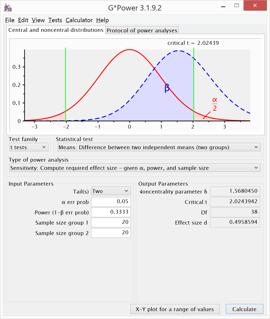
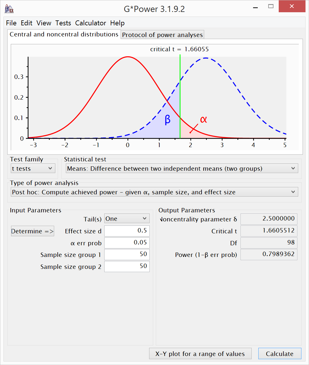
A replication with 2.5 times as many participants
(i.e., 50 per condition) has 80% power to detect and effect of 0.5 in a
one-sided t-test.
When you
design a replication study using 2.5 times the original sample size, your goal
is not to design a study that will allow you to draw correct conclusions about
the presence or absence of an effect. When you use 2.5 times the sample size of
the original study, the goal is to reject the null of a detectable effect (defined
as an effect size the original sample had 33% power for) with 80% power. Note
that in this question, the null is the assumption that d = 0.5, and the alternative hypothesis is d = 0 (a reversal of what we typically would call the null and
alternative hypothesis). If we can reject the null (d = 0.5) when testing the alternative hypothesis (d = 0), this means the replication results
are inconsistent with an effect size big enough to be detectable by the
original study, 80% of the time. In other words, with 2.5 times the sample size
of an original study, we can reject an effect size the original study had 33% power for 80% of the time, if the true effect size is 0. It has become less likely
that the effect size estimate in the original study was accurate, but we have
learned nothing about whether the effect is true or not.
Bayesian
and sequential analyses allow researchers to design high-powered studies that
provide informational value about the presence or absence of an effect efficiently.
However, researchers rarely use these methods. One reason might be that there
are no easy to use guidelines to help researchers to design a study where they
will repeatedly analyze their data.
I believe
researchers most often perform studies because they want to learn something
about the presence or absence of an effect (and not to have an 80% probability
to conclude the effect is smaller than the effect size the original study had
33% power to observe). I also worry that researchers will use the 2.5 * N rule without realizing which question
they will be answering, just because it is so easy to use without reading or
understanding Uri's paper – I’ve already seen it happen, and
have even done it myself.
Here, I
will provide a straightforward recommendation to design novel and replication
studies that is easy to implement and will allow researchers to draw
informative statistical inferences about the presence or absence of an effect. (I might work this into a future paper if people are interested, so feel free to leave comments below).
1) Determine the maximum sample size you
are willing to collect (e.g., N = 400)
2) Plan equally spaced analyses (e.g., four
looks at the data, after 50, 100, 150, and 200 participants per condition in a
two-sample t-test).
3) Use alpha levels for each of the
four looks at your data that control the Type 1 error rate (e.g., for four
looks: 0.019 at each look; for three looks: 0.023 at each look;
for two looks: 0.030 at each look).
4) Calculate one-sided p-values and JZS Bayes Factors (with a
scale r on the effect size of 0.5) at
every analysis. Stop when the effect is statistically significant and/or JZS Bayes
Factors > 3. Stop when there is support for the null hypothesis based on a JZS
Bayes Factor < 0.33. If the results are inconclusive, continue. In small
samples (e.g., 50 participants per condition) the risk of Type 1 errors when
accepting the null using Bayes Factors is relatively high, so always interpret
results from small samples with caution.
5) When the maximum sample size is
reached without providing convincing evidence for the null or alternative
hypothesis, interpret the Bayes Factor while acknowledging the Bayes Factor provides
weak support for either the null or the alternative hypothesis. Conclude that
based on the power you had to observe a small effect size (e.g., 91% power to
observe a d = 0.3) the true effect
size is most likely either zero or small.
6) Report the effect size and its 95%
confidence interval, and interpret it in relation to other findings in the
literature or to theoretical predictions about the size of the effect.
See the footnote for the reason behind the specific choices in this
procedure. You can use R, JASP, or online calculators to compute
the Bayes Factor. This approach will give you a good chance of providing support for the alternative hypothesis if there is a true
effect (i.e., a low Type 2 error). This makes it unlikely researchers will
falsely conclude an effect is not replicable, when there is a true effect.
Demonstration 1: d = 0.5
If we run 10 simulations of replication studies where the true effect
size is d=0.5, and the sample size in
the original study was 20 participants per cell, we can compare different
approaches to determine the sample size. The graphs display 10 lines for the p-values (top) and effect size (bottom)
as the sample size grows from 20 to 200. The vertical colored lines represent
the time when the data is analyzed. There are four looks after 50, 100, 150,
and 200 participants in each condition. The green curve in the upper plot is
the power for a d = 0.5 as the sample
size increases, and the yellow lines in the bottom plot display the 95% prediction
interval around a d = 0.5 as the sample
size increases. P-values above the
brown curved line are statistically different from 0 (the brown straight line)
using a one-sided test with an alpha of 0.02. This plot is heavily inspired by Schönbrodt
& Perugini, 2013.

Let’s
compare the results from the tests (both the p-values, Bayes Factors, and effect sizes) at the four looks at our
data. The results from each test for the 10 simulations is presented below.

Our
decision rules were to interpret the data as support of the presence of a true
effect when p < α, or BF > 3. If we use sequential analyses, we rely on
an alpha level of 0.018 for the first look. We can conclude an effect is
present after the first look in four of the studies. We continue the data
collection for 6 studies to the second looks, where three studies are now convincing
support for the presence of an effect, but the remaining three are not. We
continue to N = 150 and see all three remaining studies have now yielded
significant p-values and stop the
data collection. We make no Type 2 errors, and we have collected 4*50, 3*100,
and 3*150 participants per condition across the 10 studies (950 per condition,
or 1900 in total).
Based on
10000 simulations, we’d have 64%, 92%, 99%, and 99.9% power at each look to
detect an effect of d = 0.5. Bayes Factors would correctly provide support for
the alternative hypothesis at the four looks in 67%, 92%, 98%, and 99.7% of the
studies, respectively. Bayes Factors would also incorrectly provide support for
the null hypothesis at the four looks in 0.9%, 0.2%, 0.02%, and approximately
0% of the studies, respectively. Note that using BF > 3 as a decision rule
in a Neyman-Pearson theory inflates the Type 1 error rate in the same way as it
does for p-values, as Uri Simonsohn
explains.
Using N * 2.5 to design a study
If our
simulations were replications of an original study with 20 participants in each
condition, analyzing the data after 50 participants in each condition would be
identical to using the N * 2.5 rule. A study with a sample size of 20 per cell
has 33% power for an effect with d =
0.5, and the power after 50 participants per cell is 80% (illustrated by the
green power line for a one-sided test crossing the green horizontal line at 50
participants.
If we use
the N*2.5 rule, and test after 50 participants with an alpha of .05 we see we
can conclude 6 simulated studies reveal a data pattern that is surprising,
assuming H0 is true. Even though we have approximately 80% power in the long
run, in small dataset such as 10 replications, a success rate of 60% is no
exception (but we could just as well have gotten lucky, and found 10 studies
toe be statistically significant). There are 4 Type 2 errors, and have
collected 10*50 = 500 participants in each condition (or 1000 participants in
total).
It should
be clear that the use of N * 2.5 is unrelated to the probability a study will
provide convincing support for either the null hypothesis or the alternative
hypothesis. If the original study was much larger than N = 20 per condition the
study might have too much power (which is problematic if collecting data is
costly), and when the true effect size is smaller than d = 0.5 in the current
example, the N*2.5 rule could easily lead to studies that are substantially
underpowered to detect a true effect. The N*2.5 rule is conditioned on the
effect size that could reliably be observed based on the sample size used in
the original study. It is not conditioned on the true effect size.
Demonstration 2: d = 0
Let’s run
the simulation 1000 times, while setting the true effect size to d=0, to evaluate our decision rule when
there is no true effect.

The top
plot has turned black, because p-values
are uniformly distributed when H0 is true, and thus end up all over the place. The
bottom plot shows 95% of the effect sizes fall within the 95% prediction
interval around 0.
Sequential analyses
yield approximately 2% Type 1 errors on the four looks, and (more importantly) control
the overall Type 1 error rate so that it stays below 0.05 over the four looks
combined. After the first look, 53% of the Bayes Factors correctly lead to the
decision to accept the null hypothesis (which we can interpret as 53% power, or
53% chance of concluding the null hypothesis is true, when the null hypothesis
is true). This percentage increases to 66%, 73%, and 76% in the subsequent 3
looks (based on 10000 simulations). When using Bayes Factors, we will also make
Type 1 errors (concluding there is an effect, when there is no effect). Across
the 4 looks, this will happen 2.2%, 1.9%, 1.4%, and 1.4% of the time. Thus, the
error rates for the decision to accept the null hypothesis or rejecting the
alternative hypothesis become smaller as the sample size increases.
I’ve run additional
simulations (N = 10000 per simulation) and have plotted to probabilities of
Type 1 errors and Type 2 errors below in the Table below.

Conclusion
When effect
sizes are uncertain, an efficient way to design a study is to analyze data
repeatedly, and decide to continue the data collection conditional upon the
results of a statistical test. Using p-values
and/or Bayes Factors from a Neyman-Pearson perspective on statistics it is possible to make correct decision about whether to
accept or reject the null hypothesis without making too many mistakes (i.e., Type 1 and Type 2 errors). The six
steps I propose are relatively straightforward to implement, and do not require
any advanced statistics beyond calculating Bayes Factors, effect sizes, and
their confidence intervals. Anyone interested in diving into the underlying
rationale of sequential analyses can easily choose a different number or time
on which to look at the data, choose a different alpha spending function, or
design more advanced sequential analyses (see Lakens, 2014).
The larger
the sample we are willing to collect, the more often we can make good decisions.
The smaller the true effect size, the more data we typically need. For example,
effects smaller than d = 0.3 quickly
require more than 200 participants to find effect reliably, and testing these
effects in smaller sample sizes (either using p-values or Bayes Factors) will often not allow you to make good
decisions about whether to accept or reject the null hypothesis. When it is
possible the true effect size is small, be especially careful in accepting the
null-hypothesis based on Bayes Factors. The error rates when effect sizes are
small (e.g., d = 0.3) and sample
sizes are small (to detect small effects, e.g., N < 100 per condition) are relatively high (see Figure 3 above).
There will
always remain studies where the data are inconclusive. Reporting and
interpreting the effect size (and its 95% confidence interval) is always
useful, even when conclusions about the presence or absence of an effect must
be postponed to a future meta-analysis. The goal to accurately estimate effect
sizes is a different question than the goal to distinguish a signal from the
noise (for the sample sizes needed to accurately estimate effect sizes, see Maxwell,
Kelley, & Rausch, 2008). Indeed, some people recommend a similar estimation
focus when using Bayesian statistics (e.g., Kruschke).
I think estimation procedures become more important after we are relatively
certain the effect exists over multiple studies, and can also be done using
meta-analysis.
Whenever
researchers are interested in distinguishing the signal from the noise
efficiently, and have a maximum number of participants they are willing to
collect, the current approach allows researchers to design studies with high
informational value that will allow them to accept or reject the
null-hypothesis efficiently for large and medium effect sizes without making
too many errors. Give it a try.
Footnote
Obviously, all choices in this recommendation can be easily changed to
your preferences, and I might change these recommendations based on progressive
insights. To control the Type 1 error rate in sequential analyses, a spending
function needs to be chosen. The Type 1 error rate can be spent in many
different ways, but the continuous approximation of a Pocock spending function,
which reduced the alpha level at each interim test to approximately the same
alpha level, should work well in replication studies where the true effect size
is unknown because it reduces the alpha level more or less to the same alpha
level for each look. For four looks at the data, the alpha levels for the four
one-sided tests are 0.018, 0.019, 0.020, and 0.021. It does not matter which test
you perform when you look at the data. Lowering alpha levels reduces the power
of the test, and thus requires somewhat more participants, but this is
compensated by being able to stop the data collection early (see Lakens, 2014).
These four looks after 50, 100, 150, and 200 participants per condition give
you 90% power in a one-sided t-test
to observe an effect of d = 0.68, d = 0.48, d = 0.39, and d = 0.33,
respectively. You can also choose to look at the data less, or more. Finally,
Bayes Factors come in many flavors: I use the JZS Bayes Factor, with a scale r
on the effect size of 0.5, recommended by Rouder et al (2009) when one
primarily expects small effects. This keep erroneous conclusions about H0 being
true when there is a small effect reasonable acceptable (e.g., for d = 3, Type 2 errors are smaller than 5%
after 100 participants in each condition of a t-test). It somewhat reduces the power to accept the
null-hypothesis (e.g., 54%, 67%, 73%, and 77% in each of the four looks,
respectively) but since inconclusive outcomes also indicate the true effect is
either zero or very small, this decision procedure seems acceptable. Thanks to Uri
Simonsohn for pointing to the importance of carefully choosing a scale r on
the effect size.
The script used to run the simulations and create the graphs is available below:
The script used to run the simulations and create the graphs is available below:


