[The points made in this blog posts are now published: Albers, C. & Lakens, D. (2017). Biased sample size estimates in a-priori power analysis due to the choice of the effect size index and follow-up bias. Journal of Experimental Social Psychology. Read the pre-print here.]
Eta-squared (η²) and partial eta-squared (ηp²) are biased effect size estimators. I knew this, but I never understood how bad it was. Here’s how bad it is: If η² was a flight from New York to Amsterdam, you would end up in Berlin. Because of the bias, using η² or ηp² in power analyses can lead to underpowered studies, because the sample size estimate will be too small. Below, I’ll share a relatively unknown but remarkably easy to use formula to calculate partial omega squared ωp² which you can use in power analyses instead of ηp². You should probably always us ωp² in power analyses. And it makes sense to round ωp² to three digits instead of two, especially for small to medium effect sizes.
Eta-squared (η²) and partial eta-squared (ηp²) are biased effect size estimators. I knew this, but I never understood how bad it was. Here’s how bad it is: If η² was a flight from New York to Amsterdam, you would end up in Berlin. Because of the bias, using η² or ηp² in power analyses can lead to underpowered studies, because the sample size estimate will be too small. Below, I’ll share a relatively unknown but remarkably easy to use formula to calculate partial omega squared ωp² which you can use in power analyses instead of ηp². You should probably always us ωp² in power analyses. And it makes sense to round ωp² to three digits instead of two, especially for small to medium effect sizes.
Effect
sizes have variance (they vary every time you would perform the same
experiment) but they can also have systematic bias. For Cohen’s d a less biased effect size estimate is
known as Hedges’ g. For η² less
biased estimators are epsilon squared (ε²) and
omega-squared (ω²).
Texts on statistics often mention ω² is a less biased version of η², but I’ve never
heard people argue strongly against using η² at all (EDIT: This was probably because I hadn't read Caroll & Nordholm, 1975; Skidmore & Thompson, 2012; Wickens & Keppel, 2004. For example, in Skidmore & Thompson, 2012: "Overall, our results corroborate the limited previous research (Carroll & Nordholm, 1975; Keselman, 1975) and suggest that η2 should not be used as an ANOVA effect size estimator"). Because no one ever
clearly demonstrated to me how much it matters, and software such as SPSS
conveniently provides ηp² but
not εp² or ωp², I personally ignored ω². I thought that
if it really mattered, we would all be using ω². Ha, ha.
While reading
up on this topic, I came across work by Okada (2013). He
re-examines the widespread belief that ω² is
the preferred and least biased alternative to η². Keselman (1975) had shown
that in terms of bias ω²
< ε² < η². It turns out that might have been due to a
lousy random number generator and too small sample size (number of
simulations). Okada (2013) shows that in terms of bias ε²
< ω² < η². It
demonstrates that even in statistics replication is really important.
The bias in
η² decreases as the sample size per
condition increases, and it increases as the effect size becomes smaller (but not that much). Because the
size of the bias remains rather stable as the true effect size decreases, the ratio
between the bias and the true effect size becomes larger when the effect size
decreases. Where an overestimation of 0.03 isn’t huge when η² = 0.26, it is
substantial when the true η² = 0.06. Let’s see how much it matters, for all
practical purposes.
How biased is eta-squared?
Okada
(2013) includes a table with the bias for η²,
ε²,
and ω², for sample sizes
of 10 to 100 per condition, for three effect sizes. He uses small, medium, and
large effect sizes following Keselman (1975), but I have run additional simulations for the now more commonly used small (η² = 0.0099), medium (η² = 0.0588), and large (η²
= 0.1379) effects, based on Cohen (1988).
Cohen actually meant ηp² with these benchmarks (as Richardson,
2011 recently reminded me), but in a One-Way ANOVA η² = ηp². I’ve
used Okada’s R script to calculate the bias for four effect sizes (based on
1000000 simulations): no effect (η² = 0), small
(η² = 0.0099), medium (η² = 0.0588), and large (η² = 0.1379). Note
therefore that my labels for small, medium, and large differ from those in
Okada (2013). Also, formula 5 for ω² in Okada (2013) is incorrect, the
denominator should be SSt/MSw
instead of SSt/SSw.
It is a typo - the correct formula was used in the R script. The script
simulated an ANOVA with 4 groups (click to enlarge).
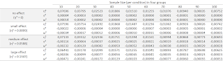
The table shows the bias. With four groups of n = 20, a One-Way ANOVA with a medium effect (true η² = 0.0588) will overestimate the true effect size on average by 0.03512, for an average observed η² of = 0.0588 + 0.03512 = 0.09392. We can see that for small effects (η² = 0.0099) the bias is actually larger than the true effect size (up to ANOVA’s with 70 participants in each condition).

The table shows the bias. With four groups of n = 20, a One-Way ANOVA with a medium effect (true η² = 0.0588) will overestimate the true effect size on average by 0.03512, for an average observed η² of = 0.0588 + 0.03512 = 0.09392. We can see that for small effects (η² = 0.0099) the bias is actually larger than the true effect size (up to ANOVA’s with 70 participants in each condition).
When there is no true effect, η² from small studies can easily give the wrong impression that there is a real small to medium effect, just due to the bias. Your p-value would not be statistically significant, but this overestimation could be problematic if you ignore the p-value and just focus on estimation.
I ran some
additional simulations with two groups (see the Table below). The difference between the 4 group and 2 group simulations shows the bias increases as the number of groups increases. It is smallest with only two groups, but even here, the eta-squared from studies with small samples are biased and this bias will influence power calculations. It is also important to correct for this bias in meta-analysis. Instead of converting η² directly to r, it is better to convert ω² to r. It would be interesting to examine if this bias influences published meta-analyses.


It is also
clear that ε² and ω² are
massively more accurate. As Okada (2013) observed, and unlike most statistics
textbook will tell you, ε²
is less biased than ω². However, they both do a good
job for most practical purposes. Based on the belief ω² was less biased than
ε², statisticians typically ignore ε². For example, (Olejnik & Algina,
2003) discuss generalized ωG², but not εG². More future
work.
Impact on A-Priori Power Analysis
Let’s say
you perform a power analysis using the observed η² of 0.0935 when the true η² =
0.0588. With 80% power, an alpha of 0.05, and 4 groups, the recommended sample
size is 112 participants in total. An a-priori power analysis with the correct
(true) η² = 0.0588 would have yielded a required sample size of 180. With 112
participants, you would have 57% power, instead of 80% power.
So there’s
that.
Even when
the bias in η² is only 0.01, we are still talking about a sample size
calculation of 152 instead of 180 for a medium effect size. If you consider the
fact we are only reporting this effect size because SPSS gives it, we might
just as well report something more useful. I think as scientists we should not
run eta-airways with flights from New-York to Amsterdam that end up in Berlin.
We should stop using eta-squared. (Obviously, it would help if statistic
software would report unbiased effect sizes. The only statistical software I
know that has an easy way to request omega-squared is Stata – even R fails us
here - but see the easy to use formula below).
This also means it makes sense to round ηp² or ωp² to three digits instead of two. When you observe a medium effect, and write down that ωp² = 0.06, it matters for a power analysis (2 groups, 80% power) whether the true value was 0.064 (total sample size: 118) or 0.056 (total sample size: 136). The difference becomes more pronounced for smaller effect sizes. Obviously, power analyses at their best give a tentative answer to the number of participants you need. Sequential analyses are a superior way to design well-powered studies.
This also means it makes sense to round ηp² or ωp² to three digits instead of two. When you observe a medium effect, and write down that ωp² = 0.06, it matters for a power analysis (2 groups, 80% power) whether the true value was 0.064 (total sample size: 118) or 0.056 (total sample size: 136). The difference becomes more pronounced for smaller effect sizes. Obviously, power analyses at their best give a tentative answer to the number of participants you need. Sequential analyses are a superior way to design well-powered studies.
Calculating Partial Omega-Squared
Here’s the
game-changer for me, personally. In power analysis, you need the partial effect size. I thought you could only calculate ωp² if you had
access to the ANOVA table, because most formulas look like this:

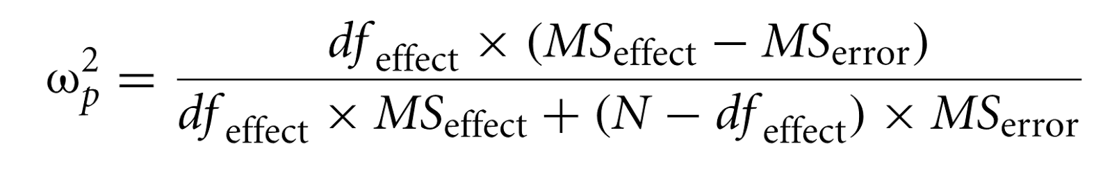
and the
mean squares are not available to researchers. But, Maxwell and Delaney (2004, formula
7.46) apply some basic algebra and give a much more useful formula to calculate
ωp² EDIT: Even more useful are the formula's by Carroll and Nordholm (1975) (only to be used for a One-Way ANOVA):

Where N is the sample size, and J the number of groups. I've done some reformulating myself, and (if I am correct, and I tried to be after double checking the results, during which I am pretty sure STATAgives used to give you epsilon squared instead of omega squared when you ask for omega squared - UPDATE: Bruce Weaver informed me this issue has been fixed) an even more convenient formula is:
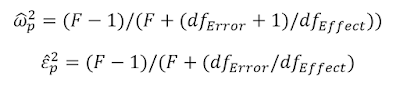
As you can see, this formula can be used if you only have the F-test, and the degrees of freedom for the effect and error. In F(1,38)=3.47 the F = 3.47, the dfeffect = 1 and the dferror = 38. That’s extremely useful. It means you can easily calculate a less biased effect size estimate from the published literature (at least for One-Way ANOVA's), and use partial omega-squared (or partial epsilon squared) in power analysis software such as G*power.
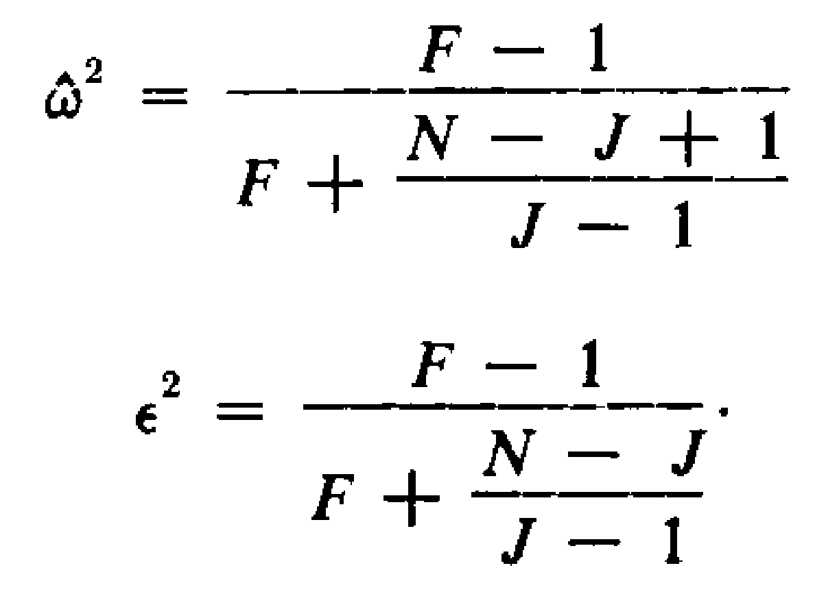
Where N is the sample size, and J the number of groups. I've done some reformulating myself, and (if I am correct, and I tried to be after double checking the results, during which I am pretty sure STATA

As you can see, this formula can be used if you only have the F-test, and the degrees of freedom for the effect and error. In F(1,38)=3.47 the F = 3.47, the dfeffect = 1 and the dferror = 38. That’s extremely useful. It means you can easily calculate a less biased effect size estimate from the published literature (at least for One-Way ANOVA's), and use partial omega-squared (or partial epsilon squared) in power analysis software such as G*power.
I’ve
updated my effect size calculation spreadsheet
to include partial omega squared for an F-test
(and updated some other calculations, such as a more accurate unbiased d formula for within designs that gives
exactly the same value as Cumming (2012) so be sure to update the spreadsheet
if you use it). You can also just use this Excel spreadsheet just for eta squared, omega squared and epsilon squared.
Although
effect sizes in the population that represent the proportion of variance are
bounded between 0 and 1, unbiased effect size estimates such as ω² can be
negative. Some people are tempted to set ω² to 0 when it is smaller than 0, but
for future meta-analyses it is probably better to just report the negative
value, even though it is impossible.
I hope this
post has convinced you of the importance of using ωp² instead of ηp²,
and that the formula provided above will make this relatively easy.
Interested in some details?
The
formulas for η², ε², and ω² are:


Here, SSt is the total sum of squared, SSb is the sum of squares between groups, SSw is the sum of
squares within groups, dfb is the degrees of
freedom between groups, and MSw is the mean sum of squares within
groups (SSw/dfw). You can find all these values in an
ANOVA table, such as SPSS provides.


G*Power
uses Cohen’s f, and will convert partial eta-squared to Cohen’s f using the
formula:
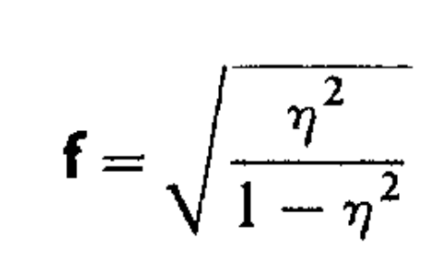
In a One-Way ANOVA, η² and ηp² are the same. When we talk about small (η² = 0.0099), medium (η² = 0.0588), and large (η² = 0.1379) effects, based on Cohen (1988), we are actually talking about ηp². Whenever η² and ηp² are not the same, ηp² is the effect size that relates to the categories described by Cohen Thanks to John Richardson who recently pointed this out in personal communication (and explains this in detail in Richardson, 2011).