A blog on statistics, methods, philosophy of science, and open science. Understanding 20% of statistics will improve 80% of your inferences.

Saturday, March 19, 2016

Who do you love most? Your left-tail or your right tail?


TL;DR: Don’t like one-sided tests? Distribute your alpha level unequally (i.e., 0.04 vs 0.01) across two tails to still benefit from an increase in power.


My two unequal tails in a 0.04/0.01 ratio (picture by my wife).


This is a follow-up to my previous post, where I explained how you can easily become 20% more efficient when you aim for 80% power, by using a one-sided test. The only requirements for this 20% efficiency benefit is 1) you have a one-sided prediction, and 2) you want to calculate a p-value. It is advisable to pre-register your analysis plan, for many reasons, one being to convince reviewers you planned to do a one-sided test all along. This blog is an update for people who responded they often don't have a one-sided prediction.

First, who would have a negative attitude towards becoming 20% more efficient by using one-sided tests, when appropriate? Neo-Fisherians (e.g., Hurlbert & Lombardi, 2012). These people think error control is bogus, data is data, and p-values are to be interpreted as likelihoods. A p-value of 0.00001 is strong evidence, a p-value of 0.03 is some evidence. If you looked at your data standing on one-leg, and then hanging upside down, and because of this you will use a Bonferroni-corrected alpha of 0.025 and treat a p-value of 0.03 differently, well that’s just silly.

I almost fully sympathize with this ‘just let the data speak’ perspective. Obviously, your p-value of 0.03 will sometimes be evidence for the null-hypothesis, but I realize the correlation between p-values and evidence is strong enough that it works, in practice, even when it is a formally invalid approach to statistical inferences.

However, I don’t think you should just let the data speak to you. You need to use error control as a first line of defense against making a fool of yourself. If you don’t, you will look at random noise, and think that a high success rate on erotic pictures, but not on romantic pictures, neutral pictures, negative pictures, and positive pictures, is evidence of pre-cognition (p = 0.031, see Bem, 2011).

Now you are free to make an informed choice here. If you think the p=0.031 is evidence for pre-cognition, multiple comparisons be damned, I’ll happily send you a free neo-Fisherian sticker for your laptop. But I think you care about error control. And given that it’s not an either-or choice, you can control error rates and after you have distinguished the signal from the noise, let the strength of the evidence speak through the likelihood function.

Remember: Type 2 error control, achieved by having high power, means you will not say there is nothing, when there is something, more than X% of the time.

Now for the update to my previous post. Even when you want to allow for effects in both directions, you typically care more about missing an effect in one direction, than you care about missing an effect in the opposite direction. That is: You care more about saying there is nothing, when there is something, in one direction, than you care about saying there is nothing, when there is something, in the other direction. That is, if you care about power, you will typically want to distribute your alpha unequally across both tails.

Rice and Gaines (1994) believe that many researchers would rather deal with an unexpected result in the opposite direction from their original hypothesis by creating a new hypothesis, than ignoring the result as not supporting the original hypothesis. I find this a troublesome approach to theory testing. But their recommendation to distribute alpha levels unevenly across the two tails is valid for anyone who has a two-sided prediction, where the importance of effects in both directions is not equal.

I think in most studies people typically care more about effects in one direction, than about effects in the other direction, even when they don't have a directional prediction. Rice and Gaines propose using an alpha of 0.01 for one tail, and an alpha of 0.04 for the other tail.

I believe that is an excellent recommendation for people who do not have a directional hypothesis, but would like to benefit from an increase in power for the result in the direction they care most about.


References

Bem, D. J. (2011). Feeling the future: experimental evidence for anomalous retroactive influences on cognition and affect. Journal of Personality and Social Psychology, 100(3), 407.
Hurlbert, S. H., & Lombardi, C. M. (2012). Lopsided reasoning: On lopsided tests and multiple comparisons. Australian & New Zealand Journal of Statistics, 54(1), 23–42. http://doi.org/10.1111/j.1467-842X.2012.00652.x
Rice, W. R., & Gaines, S. D. (1994). “Heads I win, tails you lose”: testing directional alternative hypotheses in ecological and evolutionary research. Trends in Ecology & Evolution, 9(6), 235–237. http://doi.org/10.1016/0169-5347(94)90258-5
Thursday, March 17, 2016

One-sided tests: Efficient and Underused

Researchers often have a directional hypothesis (e.g., the reaction times in the implicit association test are slower in the incongruent block compared to the congruent block). In these situations, researchers can choose to use either a two-sided test:

H0: Mean 1 – Mean 2 = 0
H1: Mean 1 – Mean 2 ≠ 0

or a one-sided test:

H0: Mean 1 – Mean 2 ≤ 0
H1: Mean 1 – Mean 2 > 0

One-sided tests are more powerful than two-sided tests. If you design a test with 80% power, a one-sided test requires approximately 79% of the total sample of a two-sided test. This means that the use of one-sided tests would make researchers more efficient. Tax money would be spent more efficiently.

Many researchers have reacted negatively to the “widespread overuse of two-tailed testing for directional research hypotheses tests” (Cho & Abe, 2013 – this a good read). As Jones (1952, p. 46) remarks: “Since the test of the null hypothesis against a one-sided alternative is the most powerful test for all directional hypotheses, it is strongly recommended that the one-tailed model be adopted wherever its use is appropriate”.

Nevertheless, researchers predominantly use two-sided tests. The use of one-sided tests is associated with attempts to get a non-significant p-value of 0.08 below the 0.05 threshold. I predict that the increased use of pre-registration will finally allow researchers to take advantage of more efficient one-sided tests, whenever they have a clear one-sided hypothesis.

There has been some discussion in the literature about the validity of one-sided tests, even when researchers have a directional hypothesis. This discussion has probably confused researchers enough to prevent them from changing the status quo of default use of two-sided tests. However, ignorance is not a good excuse to waste tax money in science. Furthermore, we can expect that in competitive research environments, researchers would prefer to be more efficient, whenever this is justified. Let’s discuss the factors that determine whether someone would use a one-sided or two-sided test.

First of all, a researcher should have a hypothesis where the expected effect lies in a specific direction. Importantly, the question is not whether a result in the opposite direction is possible, but whether it supports your hypothesis. For example, quizzing students during a series of lectures seems to be a useful way to improve their grade for the final exam. I set out to test this hypothesis. Half of the students receive weekly quizzes, while the other half does not get weekly quizzes. It is possible that, opposed to my prediction, the students who are quizzed actually perform worse. However, this is not of interest to me. I want to decide if I should take time during my lectures to quiz my students to improve their grades, or whether I should not do this. Therefore, I want to know if quizzes improve grades, or not. A one-sided test answers my question. If I decide to introduce quizzes in my lectures whenever p < alpha, where my alpha level is an acceptable Type 1 error rate, a one-sided test is a more efficient way to answer my question than a two-sided test.

If the introduction of quizzes substantially reduces exam grades, as opposed to my hypothesis, this might be an interesting observation for other researchers. A second concern raised against one-sided tests is that surprising findings in the opposite direction might be meaningful, and should not be ignored. I agree, but this is not an argument against one-sided testing. The goal in null-hypothesis significance testing is, not surprisingly, to test a hypothesis. But we are not in the business of testing a hypothesis we fabricated after looking at the data. Remember that the only correct use of a p-value is to control error rates when testing a hypothesis (the Neyman-Pearson approach to hypothesis testing). If you have a directional hypothesis, a result in the opposite direction can never confirm your hypothesis. It can confirm a new hypothesis, but this new hypothesis cannot be tested with a p-value calculated from the same data that was used to generate the hypothesis. It makes sense to describe the unexpected pattern in your data when you publish your research. The descriptive statistics can be used to communicate the direction and size of the observed effect. Although you can’t report a meaningful p-value, you are free to add a Bayes Factor or likelihood ratio as a measure of evidence in the data. There is a difference between describing data, and testing a hypothesis. A one-sided hypothesis test does not prohibit researchers from describing unexpected data patterns.

A third concern is that a one-sided test leads to weaker evidence (e.g., Schulz & Grimes, 2005). This is trivially true: Any change to the design of a study that requires a smaller sample size reduces the strength of the evidence you collect, since the evidence is inherently tied to the total number of observations. Other techniques to design more efficient studies (e.g., sequential analyses, Lakens, 2014) also lead to lower samples sizes, and thus less evidence. The response to this concern is straightforward: If you desire a specific level of evidence, design a study that provides this desired level of evidence. Criticizing a one-sided test because it reduces the level of evidence is an implicit acknowledgement that a two-sided test provides the desired level of evidence, which is illogical, since p-values are only weakly related to evidence to begin with (Good, 1992). Furthermore, the use of a one-sided test does not force you to reduce the sample size. For example, a researcher will collect the maximum number of participants that are available given the current resources should still use a one-sided test whenever possible to increase statistical power, even when the choice for a one-sided vs. two-sided test does not change the level of evidence in the data. There is a difference between designing a study that yields a certain level of evidence, and a study that adequately controls the error rates when performing a hypothesis test.

I think this sufficiently addresses the concerns raised in the literature (but this blog is my invitation to you to tell me why I am wrong, or raise new concerns).

We can now answer the question when we should use one-sided tests. To prevent wasting tax money, one-sided tests should be performed whenever:

1) a hypothesis involves a directional prediction

2) a p-value is calculated.

I believe there are many studies that meet these two requirements. Researchers should take 10 minutes to pre-register their experiment (just to prevent reviewers from drawing an incorrect inference about why you are using a one-sided test), to benefit from the 20% reduction in sample size (perform 5 studies, get one free). Also, these benefits stack with the reduction in the required sample when you use sequential analyses, such that a one-sided sequential analysis easily provides a 20% reduction, on top of a 20% reduction. You are welcome.


References

Good, I. J. (1992). The Bayes/Non-Bayes Compromise: A Brief Review. Journal of the American Statistical Association, 87(419), 597. http://doi.org/10.2307/2290192
Lakens, D. (2014). Performing high-powered studies efficiently with sequential analyses: Sequential analyses. European Journal of Social Psychology, 44(7), 701–710. http://doi.org/10.1002/ejsp.2023
Schulz, K. F., & Grimes, D. A. (2005). Sample size calculations in randomised trials: mandatory and mystical. The Lancet, 365(9467), 1348–1353.

Sunday, March 6, 2016

The statistical conclusions in Gilbert et al (2016) are completely invalid

In their recent commentary on the Reproducibility Project, Dan Gilbert, Gary King, Stephen Pettigrew, and Timothy Wilson (henceforth GKPW) made a crucial statistical error. In this post, I want to highlight how this error invalidates their most important claim.

COI: I was a co-author of the RP:P paper (but not of the response to Gilbert et al).

The first question GKPW address in their commentary is: “So how many of their [the RP:P] replication studies should we expect to have failed by chance alone?”

They estimate this, using Many Labs data, and they come to the conclusion that 65.5% can be expected to replicate, and thus the answer is 1-65.5%, or 34.5%.

This 65.5% is an important number, because it underlies the claim in their ‘oh screw it who cares about our reputation’ press release that: “the reproducibility of psychological science is quite high and, in fact, statistically indistinguishable from 100%”.

In the article, they compare another meaningless estimate of the number of successful replications in the RP:P with the 65.5 number and conclude: “Remarkably, the CIs of these estimates actually overlap the 65.5% replication rate that one would expect if every one of the original studies had reported a true effect.”

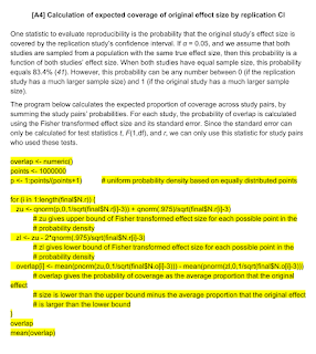
So how did GKPW get at this 65.5 number that rejects the idea that there is a reproducibility crisis in psychology? Science might not have peer reviewed this commentary (I don’t know for sure, but given the quality of the commentary, the fact that two of the authors are editors at Science, and my experience writing commentaries which are often only glanced over by editors, I’m 95% confident), but they did require the authors to share the code. I’ve added some annotations to the crucial file (see code at the bottom of this post), and you can get all the original files here. So, let's peer-review this claim ourselves.

GKPW calculated confidence intervals around all effect sizes. They then take each of the 16 studies in the Many Labs project. For each study, there are 36 replications. They take the effect size of single study at a time, and calculate how many of the remaining replications have a confidence interval around the effect size where the lower limit is larger than the effect size of the single study, or where the upper limit is smaller than the effect size. Thus, they count how many times the confidence intervals from the other studies do not contain the effect size from the single study.

As I explained in my previous blog post, they are calculating a capture percentage. The authors ‘acknowledge’ their incorrect definition of what a confidence interval is:


They also suggest they are just using the same measure we used in the RP:P paper. This is true, except that we didn’t suggest, anywhere in the RP:P paper, that there is a certain percentage that is ‘expected based on statistical theory’, as GKPW state. However, not hindered by any statistical knowledge, GKPW write in the supplementary material [TRIGGER WARNING]:

“OSC2015 does not provide a similar baseline for the CI replication test from Table 1, column 10, although based on statistical theory we know that 95% of replication estimates should fall within the 95% CI of the original results.”

Reading that statement physically hurts.

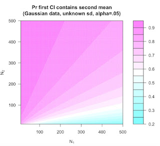
The capture percentage indicates that a single 95% confidence interval will in the long contain 83.4% of future parameters. To extend my previous blog post: There are some assumptions for this number. This percentage is only true if the sample sizes are equal (another is unbiased CI in the original studies, which is also problematic here, but not even necessary to discuss). If the replication study is larger the capture percentage is higher, and when the replication study is smaller, the capture percentage is lower. Richard Morey made a graph that plots capture percentages as a function of the difference between the sample size in the original and replication study.


The Many Labs data does not consist of 36 replications per lab, each with exactly the same sample size. Instead, sample sizes varied from 79 to 1329.

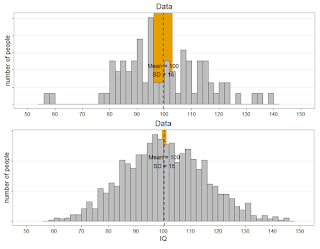
Look at the graphs below. Because the variability is much larger in the small sample (n=79, top) than in the big sample (n=1329, bottom), it's more likely that the mean in the bottom study will fall within the 95% of the top study, than it is that the mean of the top study will fall within the 95% CI of the bottom study. In an extreme case (n = 2 vs n = 100000), the mean of study n = 100000 will always fall within the 95% CI of the n = 2 study, but the mean of the n=2 study will rarely fall within the CI of the n = 100000 study, yielding a lower long-run limit of 50% for the capture percentage as calculated by GKPW.


Calculating a capture percentage across the Many Labs studies does not give an idea of what we can expect in the RP:P, if we allow some variation between studies due to 'infidelities'. The number you get says a lot about differences in sample sizes in the Many Labs study, but this can't be generalized to the RP:P. The 65.5 is a completely meaningless number with respect to what can be expected in the RP:P.

The conclusions GKPW draw based on this meaningless number, namely that “If every one of the 100 original studies that OSC attempted to replicate had described a true effect, then more than 34 of their replication studies should have failed by chance alone.” is really just complete nonsense. The statement in their press release that “the reproducibility of psychological science is quite high and, in fact, statistically indistinguishable from 100%”, based on this number, is equally meaningless.

The authors could have attempted to calculate the capture percentage for the RP:P based on the true differences in sample sizes between the original and replication studies (where 70 studies had a larger sample size, 10 the same sample size, and 20 a smaller sample size). But this would not give us the expected capture percentage, assuming all studies are true, only allowing for 'infidelities' in the replication. In addition to variation in sample sizes between original and replication studies, the capture percentage is substantially influenced by publication bias in the original studies. If we take this into account, the most probable capture percentages should be even lower. Had GKPW taken this bias into account, they would not have had to commit the world's first case of CI-hacking by only looking at the subset of 'endorsed' protocols to make the point that the 95% CI around the observed success rate for endorsed studies includes the meaningless 65.5 number.

In Uri Simonsohn’s recent blog post he writes: “the Gilbert et al. commentary opens with what appears to be an incorrectly calculated probability. One could straw-man argue against the commentary by focusing on that calculation”. I hope to have convinced the readers that focusing on this incorrectly calculated probability is not a straw man. It completely invalidates a third of their commentary, the main point they open with, and arguably the only thing that was novel about the commentary. (The other two points about power and differences between original studies and replications were discussed in the original report [even though the detailed differences between studies could not be discussed in detail due to word limitations; however, the commentary doesn’t adequately discuss this issue either]).

The use of the confidence interval interpretation of replicability in the OSC article was probably a mistake, too much based on the 'New Statistics' hype two years ago. The number is basically impossible to interpret, there is no reliable benchmark to compare it against, and it doesn't really answer any meaningful question.

But the number is very easy to misinterpret. We see this clearly in the commentary by Gilbert, King, Pettigrew and Wilson.

To conclude: How many replication studies should we expect to have failed by chance alone? My answer is 42 (and the real answer is: We can't know). Should Science follow Psychological Science's recent decision to use statistical advisors? Yes.


P.S. Marcel van Assen points out in the comments that the correct definition, and code, for the CI overlap measure were readily available in the supplement. See here, or the screenshot below:


Wednesday, March 2, 2016

The difference between a confidence interval and a capture percentage


I was reworking a lecture on confidence intervals I’ll be teaching, when I came across a perfect real life example of a common error people make when interpreting confidence intervals. I hope everyone (Harvard Professors, Science editors, my bachelor students) will benefit from a clear explanation of this misinterpretation of confidence intervals.

Let’s assume a Harvard professor and two Science editors make the following statement:
If you take 100 original studies and replicate them, then “sampling error alone should cause 5% of the replication studies to “fail” by producing results that fall outside the 95% confidence interval of the original study.”*

The formal meaning of a confidence interval is that 95% of the confidence intervals should, in the long run, contain the true population parameter. See Kristoffer Magnusson’s excellent visualization, where you can see how 95% of the confidence intervals include the true population value. Remember that confidence intervals are a statement about where future confidence intervals will fall.

Single confidence intervals are not a statement about where the means of future samples will fall. The percentage of means in future samples that falls within a single confidence interval is called the capture percentage. The percentage of future means that fall within a single unbiased confidence interval depends upon which single confidence interval you happened to observe, but in the long run, 95% confidence intervals have a 83.4% capture percentage (Cumming & Maillardet, 2006). In other words, in a large number of unbiased original studies, 16.6% (not 5%) of replication studies will observe a parameter estimate that falls outside of a single confidence interval. (Note that this percentage assumes an equal sample size in the original and replication study – if sample sizes differ, you would need to simulate the capture percentages for each study.)

Let’s experience this through simulation. Run the entire R script available at the bottom of this post. This scripts will simulate a single sample with a true population mean of 100 and standard deviation of 15 (the mean and SD of an IQ test), and create a plot. Samples drawn from this true population will show variation, as you can see from the mean and standard deviation of the sample in the plot. The black dotted line illustrates the true mean of 100. The orange area illustrates the 95% confidence interval around the sample mean, and 95% of orange bars will contain the black dotted line. For example:


The simulation also generates a large number of additional samples, after the initial one that was plotted. The simulation returns the number of confidence intervals from these simulations that contain the mean (which should be 95% in the long run). The simulation also returns the % of sample means from future studies that fall within the 95% of the original study. This is the capture percentage. It differs from (and is typically lower than) the confidence interval.

Q1: Run the simulations multiple times (the 100000 simulations take a few seconds). Look at the output you will get in the R console. For example: “95.077 % of the 95% confidence intervals contained the true mean” and “The capture percentage for the plotted study, or the % of values within the observed confidence interval from 88.17208 to 103.1506 is: 82.377 %”. While running the simulations multiple times, look at the confidence interval around the sample mean, and relate this to the capture percentage. Which statement is true?

A) The further the sample mean in the original study is from the true population mean, the lower the capture percentage.
B) The further the sample mean in the original study is from the true population mean, the higher the capture percentage.
C) The wider the confidence interval around the mean, the higher the capture percentage.
D) The narrower the confidence interval around the mean, the higher the capture percentage.

Q2: Simulations in R are randomly generated, but you can make a specific simulation reproducible by setting the seed of the random generation process. Copy-paste “set.seed(123456)” to the first line of the R script, and run the simulation. The sample mean should be 108 (see the picture below). This is a clear overestimate of the true population parameter. Indeed, the just by chance, this simulation yielded a result that is significantly different from the null hypothesis (the mean IQ of 100), even though it is a Type 1 error. Such overestimates are common in a literature rife with publication bias. A recent large scale replication project revealed that even for studies that replicated (according to a p < 0.05 criterion), the effect sizes in the original studies were substantially inflated. Given the true mean of 100, many sample means should fall to the left of the orange bar, and this percentage is clearly much larger than 5%. What is the capture percentage in this specific situation where the original study yielded an upwardly biased estimate?


A) 95% (because I believe Harvard Professors and Science editors over you and your simulations!)
B) 42.2%
C) 84.3%
D) 89.2%

I always find it easier to see how statistics work, if you can simulate them. I hope this example makes it clear what the difference between a confidence interval and a capture percentage is.


* This is a hypothetical statement. Any similarity to commentaries that might be published in Science in the future is purely coincidental.