A p-value
is the probability of the observed, or more extreme, data, under the assumption
that the null-hypothesis is true. The goal of this blog post is to understand
what this means, and perhaps more importantly, what this doesn’t mean. People
often misunderstand p-values, but
with a little help and some dedicated effort, we should be able explain these misconceptions. Below is my attempt, but if you prefer a more verbal explanation, I can recommend Greenland et al. (2016).
First, we need to know what ‘the assumption
that the null-hypothesis is true’ looks like. Although the null-hypothesis can
be any value, here we will assume the null-hypothesis is specified as a
difference of 0. When this model is visualized in text-books, or in
power-analysis software such as g*power, you often see a graph like the one
below, with t-values on the
horizontal axis, and a critical t-value
somewhere around 1.96. For a mean difference, the p-value is calculated based on the t-distribution (which is like a normal distribution, and the larger
the sample size, the more similar the two become). I will distinguish the null
hypothesis (the mean difference in the population is exactly 0) from the
null-model (a model of the data we should expect when we draw a sample when the
null-hypothesis is true) in this post.

I’ve
recently realized that things become a lot clearer if you just plot these distributions
as mean differences, because you will more often think about means, than about t-values. So below, you can see a
null-model, assuming a standard deviation of 1, for a t-test comparing mean differences (because the SD = 1, you can also
interpret the mean differences as a Cohen’s d effect size).

The
first thing to notice is that we expect that the mean of the null-model is 0: The
distribution is centered on 0. But even if the mean in the population is 0, that
does not imply every sample will give a mean of exactly zero. There is
variation around the mean, as a function of the true standard deviation, and
the sample size. One reason why I prefer to plot the null-model in raw scores
instead of t-values is that you can
see how the null-model changes, when the sample size increases.

When we collect 5000 instead of 50
observations, we see the null-model is still centered on 0 – but in our
null-model we now expect most values will fall very close around 0. Due to the
larger sample size, we should expect to observe mean differences in our sample closer
to 0 compared to our null-model when we had only 50 observations.
Both graphs have areas that are colored
red. These areas represent 2.5% of the values in the left tail of the
distribution, and 2.5% of the values in the right tail of the distribution.
Together, they make up 5% of the most extreme mean differences we would expect
to observe, given our number of observations, when the true mean difference is
exactly 0 – representing the use of an alpha level of 5%. The vertical axis
shows the density of the curves.
Let’s assume that in the figure visualizing
the null model for N = 50 (two figures up) we observe a mean difference of 0.5
in our data. This observation falls in the red area in the right tail of the
distribution. This means that the observed mean difference is surprising, if we
assume that the true mean difference is 0. If the true mean difference is 0, we
should not expect such a extreme mean difference very often. If we calculate a p-value for this observation, we get the
probability of observing a value more extreme (in either tail, when we do a
two-tailed test) than 0.5.
Take a look at the figure that shows the
null-model when we have collected 5000 observations (one figure up), and
imagine we would again observe a mean difference of 0.5. It should be clear
that this same difference is even more surprising than it was when we collected
50 observations.
We are now almost ready to address common
misconceptions about p-values, but
before we can do this, we need to introduce a model of the data when the null
is not true. When the mean difference
is not exactly 0, the alternative hypothesis is true – but what does an
alternative model look like?
When we do a study, we rarely already know
what the true mean difference is (if we already knew, why would we do the
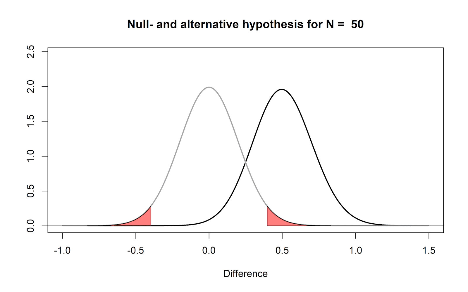
study?). But let’s assume there is an all-knowing entity. Following Paul Meehl,
we will call this all-knowing entity Omniscient Jones. Before we collect our
sample of 50 observations, Omniscient Jones already knows that the true mean
difference in the population is 0.5. Again, we should expect some variation
around this true mean difference in our small sample. The figure below again
shows the expected data pattern when the null-hypothesis is true (now indicated
by a grey line) and it shows an alternative model, assuming a true mean
difference of 0.5 exists in the population (indicated by a black line).
But Omniscient Jones could have said the
true difference was much larger. Let’s assume we do another study, but now
before we collect our 50 observations, Omniscient Jones tells us that the true
mean difference is 1.5. The null model does not change, but the alternative
model now moves over to the right.

Now, we are finally ready to address some
common misconceptions about p-values.
Before we look at misconceptions in some detail, I want to remind you of one
fact that is easy to remember, and will enable you to recognize many
misconceptions about p-values: p-values are a statement about the
probability of data, not a statement
about the probability of a theory.
Whenever you see p-values interpreted
as a probability of a theory or a hypothesis, you know something is not right.
Now let’s take a look at why this is not right.
1) Why
a non-significant p-value does not
mean that the null-hypothesis is true.
Let’s take a concrete example that will
illustrate why a non-significant result does not mean that the null-hypothesis
is true. In the figure below, Omniscient Jones tells us the true mean
difference is again 0.5. We have observed a mean difference of 0.35. This value
does not fall within the red area (and hence, the p-value is not smaller than our alpha level, or p > .05).
Nevertheless, we see that observing a mean difference of 0.35 is much more
likely under the alternative model, than under the null-model.

All the p-value
tells us is that this value is not extremely surprising, if we assume the
null-hypothesis is true. A non-significant p-value
does not mean the null-hypothesis true. It might be, but it is also possible
that the data we have observed is more likely when the alternative hypothesis
is true, than when the null-hypothesis is true (as in the figure above).
2) Why
a significant p-value does not mean
that the null-hypothesis is false.
Imagine we generate a series of numbers in
R using the following command:
rnorm(n
= 50, mean = 0, sd = 1)
This command generates 50 random
observations from a distribution with a mean of 0 and a standard deviation of
1. We run this command once, and we observe a mean difference of 0.5. We can
perform a one-sample t-test against
0, and this test tells us, with a p
< .05, that the data we have observed is surprisingly extreme, assuming the
random number generator in R functions as it should.
Should we decide to reject the
null-hypothesis that the random number generator in R works? That would be a
bold move indeed! We know that the probability of observing surprising data,
assuming the null hypothesis is true, has a maximum of 5% when our alpha is
0.05. What we can conclude, based on our data, is that we have observed an
extreme outcome, that should be considered surprising. But such an outcome is
not impossible when the null-hypothesis is true. And in this case, we really
don’t even have an alternative hypothesis that can explain the data (beyond
perhaps evil hackers taking over the website where you downloaded R).

This misconception can be expressed in many
forms. For example, one version states that the p-value is the probability that the data were generated by chance.
Note that this is just a sneaky way to say: The p-value is the probability that the null hypothesis is true, and we
observed an extreme p-value just due
to random variation. As we explained above, we can observe extreme data when we
are basically 100% certain that the null-hypothesis is true (the random number
generator in R works as it should), and seeing extreme data once should not
make you think the probability that the random number generator in R is working
is less than 5%, or in other words, that the probability that the random number
generator in R is broken is now more than 95%.
Remember: P-values are a statement about the probability of data, not a statement about the
probability of a theory or a hypothesis.
3) Why
a significant p-value does not mean
that a practically important effect has been discovered.
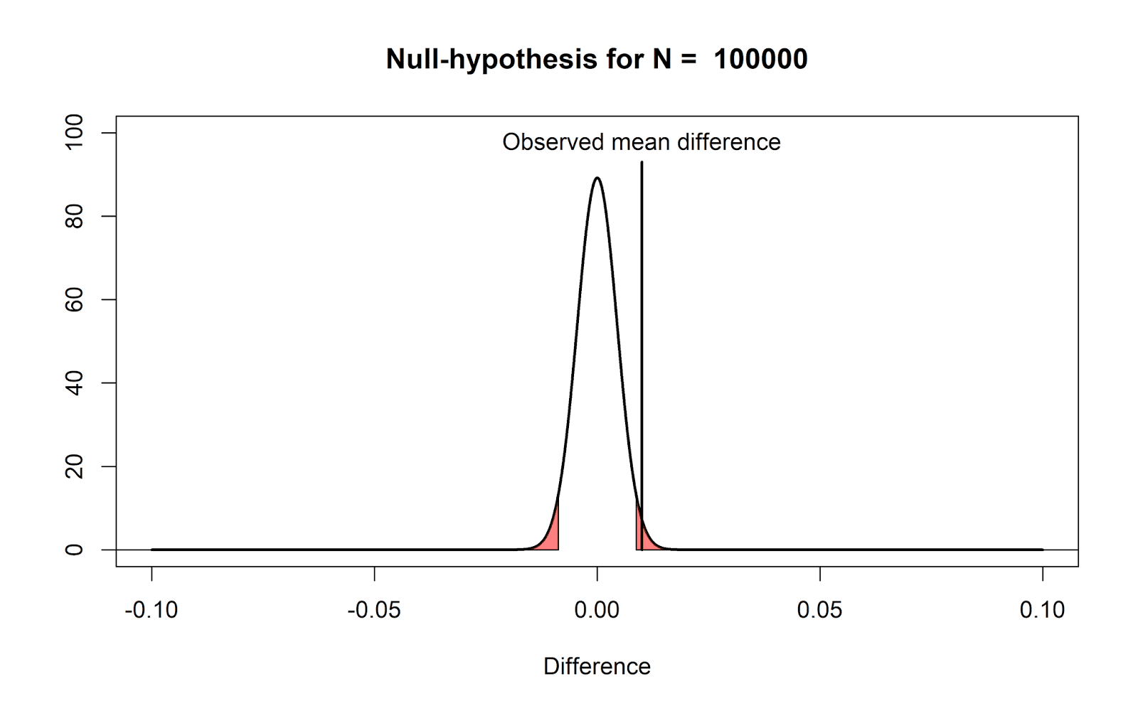
If we plot the null-model for a very large
sample size (N = 100000) we see that even very small mean differences (here, a
mean difference of 0.01) will be considered ‘surprising’. We have such a large
sample size, that all means we observe should fall very close around 0, and
even a difference of 0.01 is already considered surprising, due to our
substantial level of accuracy because we collected so much data.
Note that nothing about the definition of a
p-value changes: It still correctly
indicates that, if the null-hypothesis is true, we have observed data that
should be considered surprising. However, just because data is surprising, does
not mean we need to care about it. It is mainly the verbal label ‘significant’ that
causes confusion here – it is perhaps less confusing to think of a ‘significant’
effect as a ‘surprising’ effect (as long as the null-model is realistic - which is not automatically true).
This example illustrates why you should
always report and interpret effect sizes, with hypothesis tests. This is also
why it is useful to complement a hypothesis test with an equivalence test, so that you can
conclude the observed difference is surprisingly small if there is no
difference, but the observed difference is also surprisingly closer to zero,
assuming there exists any effect we consider meaningful (and thus, we can
conclude the effect is equivalence to zero).
4) If
you have observed a significant finding, the probability that you have made a
Type 1 error (a false positive) is not 5%.
Assume we collect 20 observations, and
Omniscient Jones tells us the null-hypothesis is true. This means we are
sampling from the following distribution:

If this is our reality, it means that 100%
of the time that we observe a significant result, it is a false positive. Thus,
100% of our significant results are Type 1 errors. What the Type 1 error rate
controls, is that from all studies we perform when the null is true, not more
than 5% of our observed mean differences will fall in the red tail areas. But
when they have fallen in the tail areas, they are always a Type 1 error. After observing
a significant result, you can not say it has a 5% probability of being a false positive.
But before you collect data, you can say you will not conclude there is an effect,
when there is no effect, more than 5% of the time, in the long run.
5) One
minus the p-value is not the probability
of observing another significant result when the experiment is replicated.
It is impossible to calculate the probability that an
effect will replicate, based on the p-value,
and as a consequence, the p-value can
not inform us about the p-value we
will observe in future studies. When we have observed a p-value of 0.05, it is not 95% certain the finding will replicate. Only
when we make additional assumptions (e.g., the assumption that the alternative
effect is true, and the effect size that was observed in the original study is
exactly correct) can we model the p-value
distribution for future studies.
It might be useful to visualize the one very
specific situation when the p-value does provide the probability that
future studies will provide a significant p-value
(even though in practice, we will never know if we are in this very specific situation).
In the figure below we have a null-model and alternative model for 150
observations. The observed mean difference falls exactly on the threshold for
the significance level. This means the p-value
is 0.05. In this specific situation, it is also 95 probable that we will
observe a significant result in a replication study, assuming there is a true effect as specified by the alternative model.
If this alternative model is true, 95% (1-p)
of the observed means will fall on the right side of the observed mean in the
original study (we have a statistical power of 95%), and only 5% of the
observed means will fall in the blue area (which contains the Type 2 errors).

This very specific situation is almost always not your reality. It is not true when any other alternative
hypothesis is correct. And it is not true when the the
null-hypothesis is true. In short, the p-value basically never, except for one very specific situation when the alternative hypothesis is true and of a very specific size you will never know you are in, gives the probability that a future study will once again yield a
significant result.
Conclusion
Probabilities are confusing, and the interpretation
of a p-value is not intuitive. Grammar
is also confusing, and not intuitive. But where we practice grammar in our education
again and again and again until you get it, we don’t practice the interpretation
of p-values again and again and again until you get it. Some repetition is probably needed. Explanations
of what p-values mean are often verbal,
and if there are figures, they use t-value
distributions we are unfamiliar with. Instead of complaining that researchers don’t
understand what p-values mean, I think we should
try to explain common misconceptions multiple times, in multiple ways.

Daniel Lakens, 2017